All About Google Sheets’ Drop Down Lists – From Constructing Them To Color-Coding

Google Sheets is a great tool for organizing and analyzing data, especially when it is team-based work you’re talking about. However, sometimes your teammates may enter data that is misspelled or has some other error. In such a case, the analysis can end up faulty, especially when it is large amounts of data one is dealing with.

To avoid making such mistakes for repeated values, Google Sheets offers an amazing option. This option, called the Google Sheets drop down list or menu, allows you to set up drop down menus for your data that you or your team members can use by simply picking one from the specified list of options, allowing you to control the data that enters a cell.

What is a Google Sheets Drop Down List?

To elaborate better, here’s an example – think of a to-do list that you made for yourself or your team. Now, in the Google Sheet, you have specified all the tasks against each team member’s name. During each phase of the task, you and your team-mates are required to fill in the Google Sheets column accordingly from the options of “To be started”, “In progress”, and “Completed”.

Now, instead of having to fill in each cell, for each task manually (or type in the entire thing), they can just select one of the three options from the Google Sheets drop down list. Working in this manner also removes any chance of typing errors because instead of typing something out in a hurry, you can just click on the option you want.

This will prevent you from having to go through each cell correcting typos, before trying to count the number of tasks to be started, in progress, or the ones that are completed.

Google Sheets drop down lists are thus a simple but effective way of not only making data more homogenous and accurate but also for saving time.

How to make a Google Sheets Drop Down List?

There are two ways to make a Google Sheets drop down list. These are:

• Using a range of cells
• Manually entering the item for the list

We will discuss both the methods in detail, explaining them both step by step, however, before we move on to that, first let’s understand what data validation is and how the different data validation options offers to help us create Google Sheets drop down lists.

What is Data Validation?

Data validation is a feature offered by Google Sheets that helps us keep our data in check. As discussed above, it makes sure no data with an error enters our Google Sheet, thereby, messing up our analysis.

a. Criteria

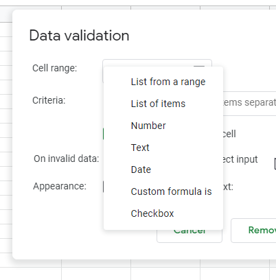
Google Sheets, for data validation, offers six options for criteria that we will discuss separately.

These are:

• List from a range
• List of items
• Number
• Text
• Date
• Custom formula is
• Checkbox

The first two options “List from a range” and “List of items” are used for Google Sheets drop down menus.

“Number” makes sure that in the specified cell only a specific number or only a number in a specific range can be entered. “Text” and “Date” work in the same way.

In “Custom formula is” a custom formula with any condition can be entered.

For all of these, you can specify your conditions, and Google Sheets will make sure that the data entered follows those conditions.

The last one reduces the need for Yes/No or similar texts and introduces a simple check box system that the user can select or deselect.

b. On Invalid Data

A common confusion is deciding between the “Show warning” and the “Reject Input” options. To pick one is entirely dependent on the admin of the Google Sheet. If the data can be fixed later, you may go with the “Show warning” option, which displays a small red tag on the top right corner of the cell for invalid data.

If absolutely no mistake at all is tolerable, then the “Reject Input” option may be picked which won’t allow the user to move forward with any error in the cell, and until they fix it.

Now that data validation has been discussed, let’s move on to the two methods of making a Google Sheets drop down list using the two methods discussed above.

Method 1 – Making a Google Sheets Drop Down List using a Range of Cells

This is the simpler option of the two, and all you need to do is to have the data which you want to be included in your list in a group of cells.

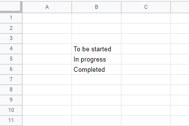
For example, let’s suppose that the three options that we want in our data are (as discussed in the previous example):

• To be started
• In progress
• Completed

Step 1:

Input these statements in three separate cells on your Google Sheet.

Step 2:

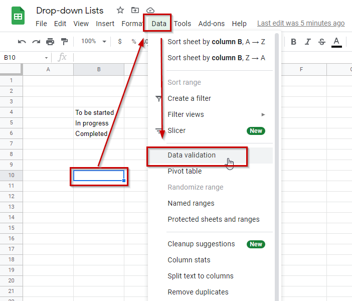
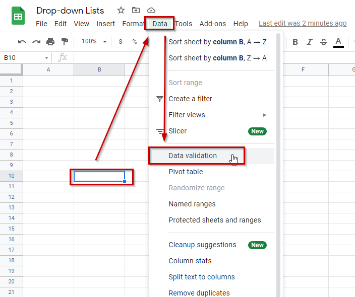
Decide in which cell you want your Google Sheets drop down list to be displayed, and then select that cell. Let’s assume that cell to be B10 in our example. Click on B10.

Step 3:

Now, from the menu bar on the top, go to “Data”, and then, from the dropdown list displayed, click on “Data Validation”.

Step 4:

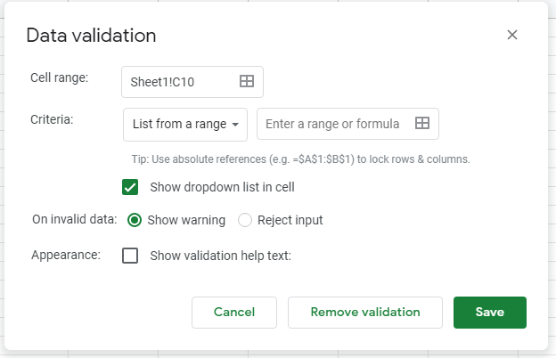
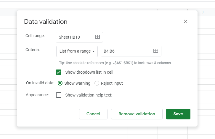
The “Data validation” set-up or dialog box will pop up in the center of your screen. This will give you a bunch of options, some of which have been discussed above under the “Data validation” topic. Over here just make sure your cell range, and criteria etc. are correct.

Cell range here, in our example, will be B10 – the cell in which our Google Sheets drop down list is to be displayed, and the criteria must be set to “List from a range”. In the criteria section, in the space that reads “Enter a range or formula”, either enter “B4:B6”, or simply select these three cells with your cursor for google sheets to automatically list them as a formula.

Make sure the “Show dropdown list in cell” option is checked.

The other next two options are dependent on whatever your preference is. The first option is for deciding what to do if a user enters a value that isn’t from one of the drop down list options, and the second one acts as a guide for the user where you can enter a help text such as “Please select one of the options from the Google Sheets drop down list”.

Step 5:

Click on “Save” and you’re done!

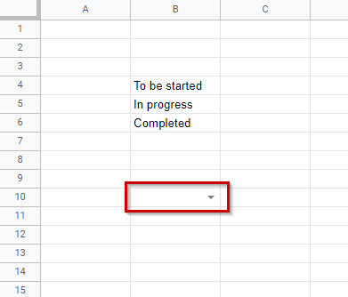
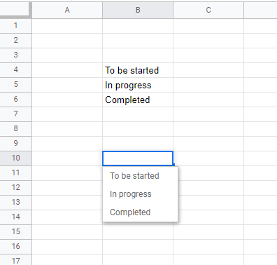
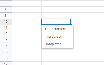
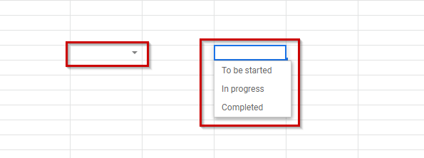
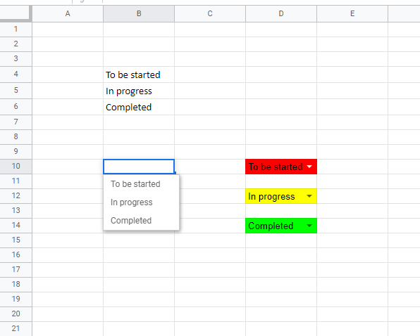
The Google Sheets drop down list can be seen here with all our accessible options from “To be started” to “Completed”.

This is what the dropdown list looks like now. You can pick and select from one of the three options, and you can also start typing it in for Google Sheets to automatically pick the matching option(/s) for you, according to your input. For example, if you enter “C”, Google Sheets will automatically show you the option(/s) starting with the letter “C” which in this case is “Completed”.

Method 2 – Making a Google Sheets Drop Down List by Manually Entering Items for the List

The second method for constructing a google sheets drop down list is almost the same, with a small difference that changes the way you go about making your list.

Step 1:

Select the cell you want your list to be displayed in. Let’s select B10.

Step 2:

Go to the “Data” option from the toolbar and then to “Data validation”.

Step 3:

In the data validation dialog box that has now appeared, in the options for “Criteria”, click on the dropdown list to see a number of different available options.

From here choose “List of items”. In the space next, enter the items you want for your Google Sheets drop down list, separated by a comma.

This is what your text will look like:

And this is how you will enter all your drop down list options:

Step 4:

Click on “Save” to successfully get your dropdown list onto your Google Sheet.

How to Modify your Google Sheets Drop Down List

Changing the Google Sheets drop down list, or any other sort of data validation setting is very simple and quick. First, let’s see how to modify a drop down list created using the “List from a range” option.

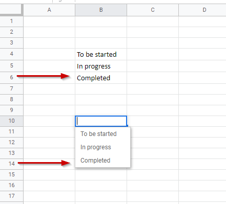
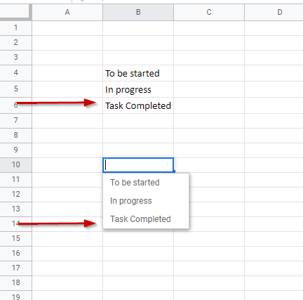
This is very simple. All you need to do is to edit the value in the originally selected range for the dropdown list, and the list will get updated automatically. Here is a before and after.

Before:

After:

For other edits as well as to modify data manually entered under the “List of items” option, just go to the “Data” option from the toolbar and then to “Data validation” from the appearing drop down menu. Upon the opening of the dialog box, edit whatever you want to edit, whether that is content-related, criteria, or cell range, etc. Cell range changes refer to changing, adding in, or removing from the original list of cells (only used for the first method of drop down list creation).

Once done, simply press “Save” for the settings to get applied.

How to Remove or Delete a Google Sheets Drop Down List

Removing a Google Sheets drop down list from a cell is very easy. All you need to do is follow these steps:

• Begin by clicking on your drop down list cell.
• Then open the “Data validation” dialog box through the same “Data” to “Data validation” step.
• Here, just click on “Remove Validation” for your selected cell to be removed from the data validation or drop down list settings.

How to Copy a Google Sheets Drop Down List

To copy a Google Sheets drop down list is also very simple – you just need to apply just the age-old Control + C and Control + V method. These are the steps you need to follow:

• Go to the cell with the drop down menu.
• Either press Control + C on your keyboard, or right click with your mouse on the cell and click on “Copy” from the drop down menu.
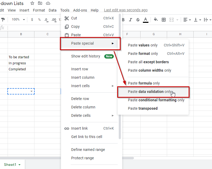
• Now go to the second location, right-click your mouse, and from the pop-up, go to “Paste special”. From here, go to the option of “Paste data validation only” and click it.

• Now your Google Sheets drop down list will be in two locations as indicated by the little arrows.

You may also Ctrl + X and then Ctrl + V to cut and paste, removing your list from the original location. If you cut and paste data validation through the paste special option, then it won’t be removed from the original location, and you will still need to remove validation from one cell through the data validation dialog box.

How to Color-Code your Google Sheets Drop Down List Options

Color coding makes the data analysis much more simple for Google Sheets’ users, and further reduces chances of error, by making the users’ selections more obvious to them. Such as a simple green box could mean “Completed” and red could mean “To be started” whereas the option of “In progress” would be an obvious yellow.

For the purpose of color-coding, we use conditional formatting.

Let’s color code the example we’ve been studying till now. Here, we will go with

1. Red for “To be started”
2. Yellow for “In progress”
3. Green for “Completed”

For color coding, you can follow these simple steps:

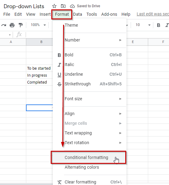
• First, you need to go to the “Format” option in the top menu bar.
• From the drop down menu list, select “Conditional formatting”.

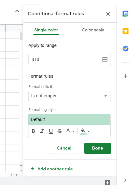
• Here, these settings’ options will appear on the right side of the screen.

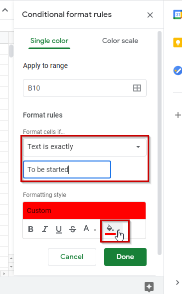
• Click on the “Format cells if…” option and from its dialog box, go to “Text is exactly”, then in the blank space below it enter “To be started”.
• Change the color through the fill color option. Since we decided on red for “To be started”., we will select red here.
• You can also change the formatting style of the drop down list options from this editing box as well.

• Once you have selected your desired overall look from the Google Sheets drop down list, press “Save”.
• Repeat this process for the other two options, with the colors yellow and green for them.
• This is what the sheet will look like when you select each of the individual options from your Google Sheets drop down menu.