Boost Productivity with 5 Google Sheets FILTER Tips

Let’s face it – looking at massive amounts of data on a spreadsheet can be a tad bit distressing. It worsens when you have to look for one specific thing in a sea of similar ones on the whole of your spreadsheet. For situations like this, google sheets offers features and functions to filter out data, from data, in the most efficient ways.
To allow users to filter data, there are two methods provided by google sheets. These are:
- The filter option
- FILTER function
Lets start with the simpler option first.
Contents
The filter option:
The google sheets filter option is a super easy feature that comes with a plethora of options to filter according to. Let’s first go over the basics of this feature, with an example.
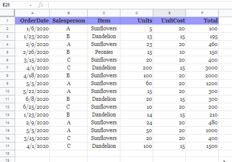
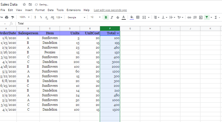
Lets assume that this is our sample data.
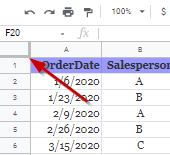
First off, you need to select your data set that you want to filter specific data from. If you want to filter off the entire sheet, just click on the rectangle where the row and column headers meet.
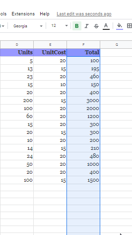
For this example, lets filter from the total sale column.
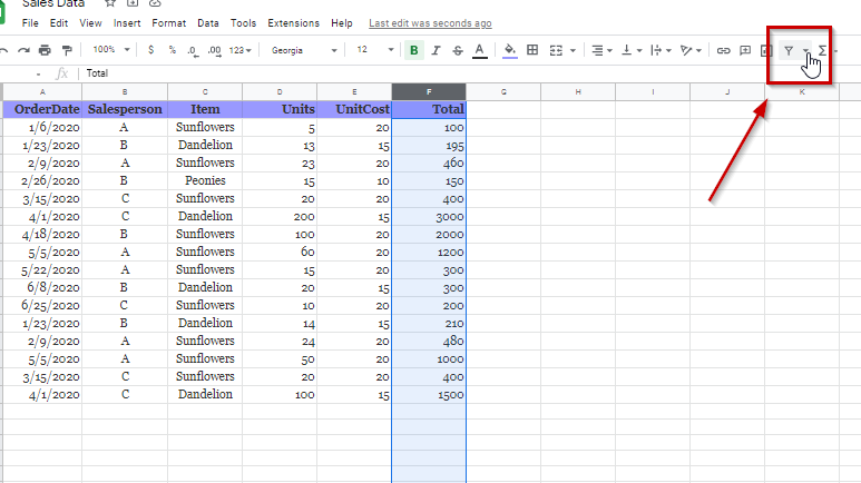
Now, hover to the toolbar and go to the second last option with the filter symbol that reads “Create filter” upper being hovered over. Click on it.
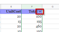
Now click on the three sort/filter lines on the right, inside the top-most cell of your selected column.
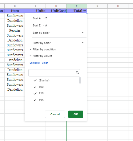
Clicking on it will display the google sheets filter options.
Here, we get a number of options. Lets start form the top.
Sort A -> Z:
This option sorts all of the selected data in ascending order, from A to Z, or for numbers, in their increasing order.
Lets test it out on our column C..
Before:
After:
Sort Z -> A:
This one does the opposite of “Sort A -> Z” and the cells are ordered in descending order. Lets test this one out on column D which contains numerical data.
Before:
After:
Sort by color:
Sort by color allows you to sort data based on either cell fill color, or test color.
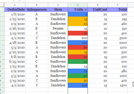
For example lets say we have different colors for our cells like this
Now, google sheets filter option here lets us filter our data according to colors by organizing the same colored cells together.
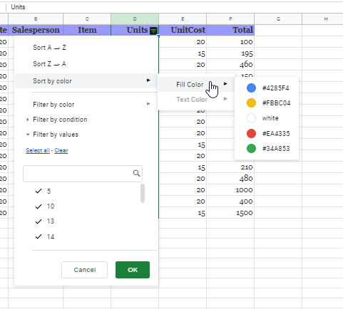
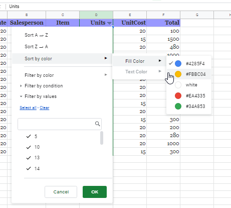
The sort by fill color option will now be activated, as our sleccted cell range has some cells with fill colors. However, since there is no colored text, the option for sorting by text color is still greyed.
Hovering over or clicking “Fill color” will display a list of all the colors used in the selected range. Select the first one, and google sheets will organize all cells with #4285F4 color together.
Now, lets select #FBBC04 alongside the already selected color.
Now, this will be the outcome.
Similarly the rest of the colors, too, can be selected one after another to arrange all the cells in the column.
Filter by color:
The “Filter by color option” allows users to not only organize the same colored cells together but also to hide all the other cells.
Let’s start with the following column as our example.
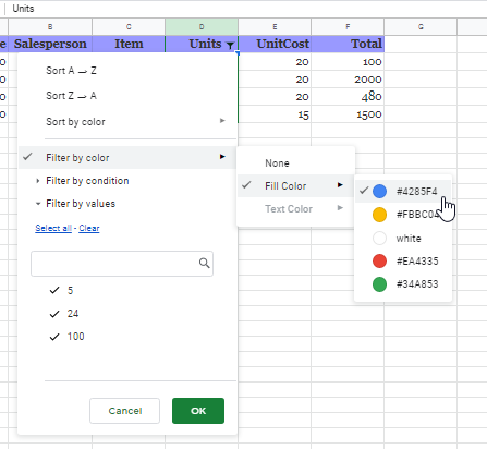
Now, we go to head cell of the column, and then to “Filter by color”, go to “Fill Color”, and select a color. Lets select #4285F4.
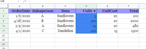
The google sheets filter option will display the following now.
Here, too, the same steps can be followed to filter out cells with each of the rest of cell fill colors.
Since we have moved to the more specific “Filter by …” options after the “Sort by …” options under the google sheets filter options, the top cell of the column displayed a filter symbol instead of the sort symbol.
Filter by condition:
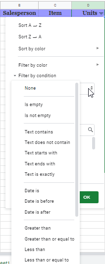
Filter by condition offers a number of defined conditions for you to apply onto your data to arrange.
Lets go over these one-by-one.
Is empty: The “Is empty” option will only display the rows that have empty cells in the selected column. This will be the opposite if a row is selected instead of a column. If no cell is empty, then no row will be displayed.
Is not empty: The “Is not empty” option only displays filled cells, as the title implies.
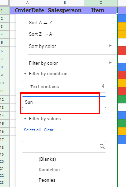
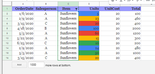
Text contains: This is google sheets filter allows to highlight cells that contain defined character(/s) in them. For example, looking for “Sun” will display both “Sun” and “Sunflower” containing cells.
Here, you can search for characters, values, as well as for formulas.
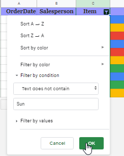
Text does not contain: Text does not contain will display the exact opposite of what text contains will display.
Lets search for “Sun” here, too.
The outcome we get will be,
Text starts with: With this, you can filter out from the entirety of your data, all the cells that start with a particular value.
Text ends with: Here, we define the ending value for google sheets filters to work according to.
Text is exactly: The condition “text is exactly”, as implies, searches for exact values. With this, searching for “Sun” will only show “Sun”, and never “Sunflower”.
“Date is”, ”Date is before”, ”Date is after”:
This three options are all together based on dates.
For ease, these conditions have auto-defined dates relative to the day you’re working on your google sheets filters. These include the following:
The first one “Date is” allows you to find specific dates. For example to find orders placed on 5/5/2020 we will use this option, and the displayed result will be,
The same procedure can be followed for using ”Date is before” and ”Date is after” for the implied purposes.
Conditions for numerals:
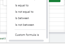
The next nine options are specific for numerals. These include,
The first eight are simple and filter data based on qualities of equivalence, being greater than, being smaller than, and graduation. The last one allows users to define specific formulas and having their data filtered accordingly. The formulas can be for anything from sums and differences to larger more complex mathematical or statistical operations.
Filter by values:
This option is probably the simplest one, if you have simple data with less categories. The “Filter by values” feature displays a list of all the different values present in each of the individual cells in the selected range. Users can check and uncheck the values to filter them. Unchecked values are filtered out, whereas the checked values are displayed.
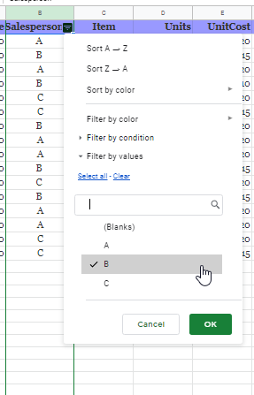
For example, if we only want to see the sales made by the Salesperson B, we will use this option, as our preference.
Uncheck all the options except B and click on “OK”.
Tip: Use the “Select all”, and “Clear” options for ease of checking and unchecking values if you have more of them.
The displayed data will be,
How to disable the filter option:
To disable the filter option, you just need to go to back to the original filter symbol position on the tool bar and hover over it. If you have filters activated, it will automatically display “Remove filters” upon being hovered over. Click on it, and it’ll remove all the applied filters.
FILTER function
The FILTER function is a google sheet function that can be applied to a cell to filter a dataset selected in a range of cells in the document based on certain conditions; the concept here is the same as the toolbar filter option, however, the filter function is more dynamic, and the filtered values change if there is a corresponding change in the selected data set. This has great applications for interactive sheets, e.g., data organization, reports etc. However, if your search range does not fit any value that satisfies the defined condition, then a simple error message “#N/A” will be displayed.
Syntax:
The filter function in google sheets has a very basic and simple syntax.
=FILTER (range, condition1, [condition2,] …)
Here,
‘Range’ is your selected range of cells among which the defined condition will be looked for in your document.
Condition1 refers to the array, column, or row that is equal in length and width as of the “range” that will return the values for TRUE or FALSE.
Condition2 is an optional additional array, row, or column that also should have the same dimensions as the range. It is applied as the second condition for the function and also returns an array of TRUEs or FALSEs.
If you use only one condition in your function formula, obviously, results for the one satisfying the condition will be filtered out. However, if you apply both conditions, only results satisfying both conditions will be filtered out.
Filtering Data based on a single condition:
As previously mentioned, if you want to filter out data based on only one condition you will use,
=FILTER (range, condition1)
Lets understand this with this example,
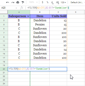
Here, lets filter out all cells that read “Dandelion”
Click on any empty cell with ample space of empty cells around it; if there aren’t enough empty cells around google sheets filter function will return the error “REF!”. Click on the cell and type in the FILTER function formula.
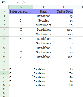
=FILTER(A2:C17,B2:B17=”Dandelion”)
Click Enter.
Here, the formula will work the same if we refer to a cell containing the word “Dandelion”
For example, our result will be the same even if we use the formula,
=FILTER(A2:C17,B2:B17=B17)
Filtering Data based on multiple conditions (AND Condition):
To find the results that satisfy two or more conditions with both of them satisfied, we apply the AND method with the following formulae,
Two conditions: =FILTER(range, condition1, condition2)
n number of conditions: =FILTER(range, condition1, condition2, condition3, …, condition)
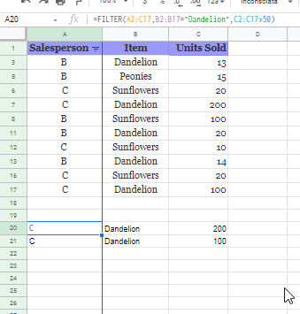
In order to find sales of Dandelions with sales over 50 units we will use the following formula,
FILTER(A2:C17,B2:B17=”Dandelion”,C2:C17>50)
The result will be,
Filtering Data based on multiple conditions (OR Condition):
Here, we will understand using the filter data according to two conditions where either one of them is satisfied.
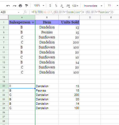
Let’s find sales of Dandelion flowers as well as those of Peonies.
=FILTER(A2:C17,(B2:B17=”Dandelion”)+ (B2:B17=”Peonies”))
Filter Top-most or bottom-most Records Based on Value:
One amazing feature of the google sheets FILTER function is that it even allows you to filter out any number of top values in order of the data stored.
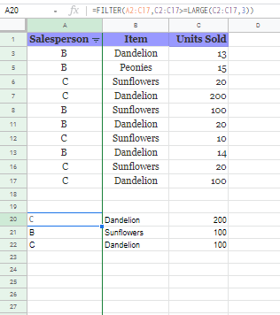
For example, lets try to find the top 3 sales of flowers from our data.
We will use the formula,
=FILTER(A2:C17,C2:C17>=LARGE(C2:C17,3))
Here, we looked for only top 3 values. By simply, substituting the last “3” in the formula to any other number, we can generate a list of that number of top sales.
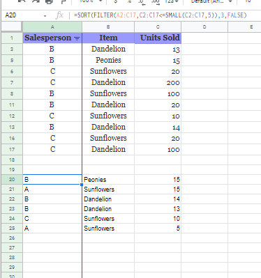
In the same way, we can also find the least or bottom-most records. Let’s look up the 5 least units of flowers sold.
The formula will have LARGE substituted by SMALL, and > substituted by < to look for lowest numbers.
How to SORT your filtered data:
Now, as previously mentioned, the filtered data, or the result here, on google sheets is always displayed in the exact order of the original data set.
Sometimes, however, that is not what we want. For example, we might want our filtered data in increasing order. For this purpose, we use the SORT function alongside the FILTER function.
Let’s try to arrange the bottom 5 values we filtered in descending order. For this, we will use the formula,
=SORT(FILTER(A2:C17,C2:C17<=SMALL(C2:C17,5)),3,FALSE)
Here, the SORT function encapsulates the FILTER function, and hence takes whatever result the FILTER function provides and sorts it into the desired order. In the formula above, the last entry, “FALSE” denotes arrangement in descending order. Replacing “FALSE” with “TRUE” would arrange the data from the highest value to the lowest in ascending order. Even leaving it blank would return the data in ascending order.
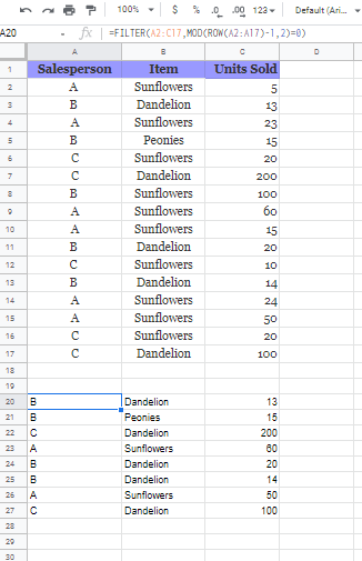
Filter all even or odd numbered rows or rows at intervals:
In order to achieve this goal, we use the formula,
=FILTER(A2:C17,MOD(ROW(A2:A17)-1,2)=0)
Here, within the FILTER function we incorporate two different functions – these are the MOD and the ROW functions. The ROW function collects the numbers of all the rows and keeps subtracting 1 from them, starting from row 2. Encapsulating the ROW function is the MOD function which checks for the condition provided by the ROW function. After the MOD operator has checked, it returns TRUE for even-numbered rows and FALSE for odd-numbered rows. This FALSE and TRUE results array is combined and utilized by the FILTER function to give the final result.
Hence, the result of the above-mentioned formula will be,
Here, the 0, in the end, refers to the odd numbers, and to get even rows’ results, we can substitute the 0 in the formula to 1.
The 2, within the ROW function, refers to skipping one row or column. If we change it to 3, we will get every third row or column.
FILTER function for when working with multiple sheets:
The google sheets FILTER function can be used to essentially combine specific data from multiple google sheets into one. For this purpose, we use a simple formula, that follows the syntax,
={FILTER({sheet#1-range},LEN({sheet#1-range-first-column})>0); FILTER({sheet#2-range},LEN({sheet#2-range-first-column})>0);…}
Here,
{sheet#1-range}refers to the data range from the first sheet and includes the title row
{sheet#2-range}refers to the data range from the second sheet and does not include the title row to ensure only one title row in the combined result
{sheet#1-range-first-column}refers to the first column of the selected data range from the first sheet.
{sheet#2-range-first-column}refers to the first column of the second sheet’s selected data range.
LEN function and the included entries signify the blank rows that are to be skipped. Not including the LEN function here would lead to the resulting filter having all the empty rows in the main sheets merged with the selected and filtered data into the combined result.
Google Sheets’ FILTER function FAQs:
Q. What happens if there is no match, for the desired condition, in our data?
A. In case Google Sheets cannot locate the appropriate answers to our questions due to their absence in our provided data, an error message of “#N/A” is displayed. This can happen when using the Google Sheets filter function to search for specific data. Hover over to the small red flag on the top right corner of your cell and there “No matches are found in the FILTER evaluation” will be displayed, indicating that the filter did not find any matching data.
Q. What if I want to FILTER rows and columns simultaneously?
A. Mixing up the conditions in a Google Sheets filter function can result in an error message. Trying to do this would result in an error message that says something like “Formula parse error.” When this happens, you can hover over the red flag in the error message cell to get more information about why the error exists. This is a helpful feature of the Google Sheets filter function that can help you troubleshoot and correct errors in your formula. So, when using the Google Sheets filter function, it’s important to pay close attention to the conditions and ensure that they are set up correctly to avoid formula errors.
Q. What if I want to filter my filtered results?
A. If you do not want the result as an array when using the Google Sheets filter function, you can simply copy your results and paste them as values and then apply a filter. However, if you still want to use the filter function on an array, you can apply a filter on a filter function. Keep in mind that using the VLOOKUP function may be a better option when working with larger datasets or when you need to look up specific values in a table. So, when using the Google Sheets filter function, you have multiple options to manipulate the data and achieve your desired result.
Q. Can I save my FILTER views?
A. Yes, if different people are sharing the same sheet as viewers, especially, you might want to have your own views saved for your convenience. For this, simply go to “Data” in the toolbar, click on “Filter Views”, and “Save as filter view” to save your filters by their own titles. To access your saved filters, go by the same steps again and you’ll find your saved filters.
h/t: SheetGO
