How to make data arrangement on google sheets simple and quick?
 Image Source: Google
Google Sheets is a service provided by Google that allows its users to assemble any kind of data in a neat and organized manner. It is especially used in the workplace where heaps of data have to be stored for decision-making purposes. However, if you have an entire Google Sheet full of data, the last thing you’d want to do would be to look at it and try to analyze it. No matter how organized it is, trying to make sense of the Google Sheet at the first glance can be quite difficult, not to mention intimidating.
In this article, we are going to tell you how to alphabetize in Google Sheets so you can have a well-organized set of data and as a result, be better able to go through the contents.
Luckily, Google Sheets offers extensive data storage options for its users. Let’s say you have, in multiple rows, data listing the population details of certain cities. If this data has many rows and columns, going through the data to find a specific city’s province or population can be a hard task. Such an issue can be resolved by a simple but amazing option that Google Sheets offers. With this, you can arrange a certain column, your entire data set, or any number of selected columns in a defined order which may be alphabetical or the reverse.
Contents
How to Alphabetize in Google Sheets?
With google sheets, you can alphabetize any range of cells, from a single column to however many you want. Let’s start with alphabetizing a single column first.
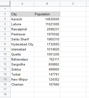
Suppose that we have the following Google Sheet containing a list of cities with their respective populations as our data.
Our goal here is to make the entire list of cities be arranged in alphabetical order. There are two methods of alphabetizing data in Google Sheets; the first one is according to the SORT function, and the second function is based on google sheets’ build in sorting options. Here, we will be discussing both methods.
1. How to Alphabetize in Google Sheets Using the SORT Function
Let us first try our hand at alphabetizing our data by using the SORT function offered by Google Sheets. Understandably so, we will be using a designated formula for this function. But first, let’s discuss what the SORT function is.
What is the SORT Function?
The SORT function sorts the data in ascending or descending order. It is an array, which means that the number of cells in your original selection will be exactly the same as the number of cells that will be taken up in your Google Sheet after the formula has been input and entered. You won’t be able to add, remove, or edit any cell.
What is the Syntax for the SORT Function?
The syntax for the SORT function is very simple:
=SORT(range, sort_column, is_ascending, [sort_column2, …],[is_ascending2, …])
In this syntax, each word represents the following:
- Range: Range here refers to the entire unorganized data that is to be sorted by the SORT function.
- Sort_column: This is the index number in the selected range of the column that contains values according to which the selected range is to be sorted. This may or may not be in the selected range.
- Is_ascending: This refers to the order in which the content is to be sorted. TRUE sorts the data in ascending order, and FASLE sorts the data in descending order.
- sort_column2, is_ascending2: These are optional, for when the user wants to add more columns to be sorted.
Let us now apply this function to our example of a single column:
To do so, select any random empty cell and in it enter your formula. Note that if you fail to mention either true or false in your syntax, Google Sheets automatically orders the data to sort itself in ascending order.
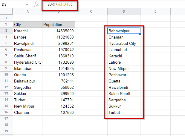
So, in order to arrange only the names of the cities in order, enter simply:
=SORT(A3:A16)
A3:A16 can also be selected manually by dragging your cursor across these cells.
Enter the formula and press enter. The result will be displayed.
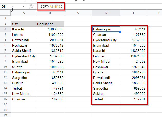
Let’s arrange the whole table now – populations against the cities listed in order.
Here, in the same D3 cell, we will enter the same formula, except with the rage A3:B16. The results will be displayed as shown:
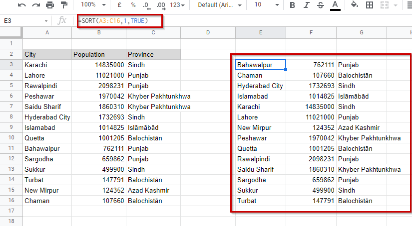
The same will work with three or more columns too. All you have to do is keep changing the range of cells accordingly. In this example, we have added a third column of provinces and have changed the range to incorporate this column as well. And in this way, you can sort out multiple columns.
Our new formula has become:
=SORT(A3:C16,1,TRUE)
Note the “1” in the syntax? This 1 represents the first column of the range i.e., A and it tells Google Sheets to arrange the entire table according to this column.
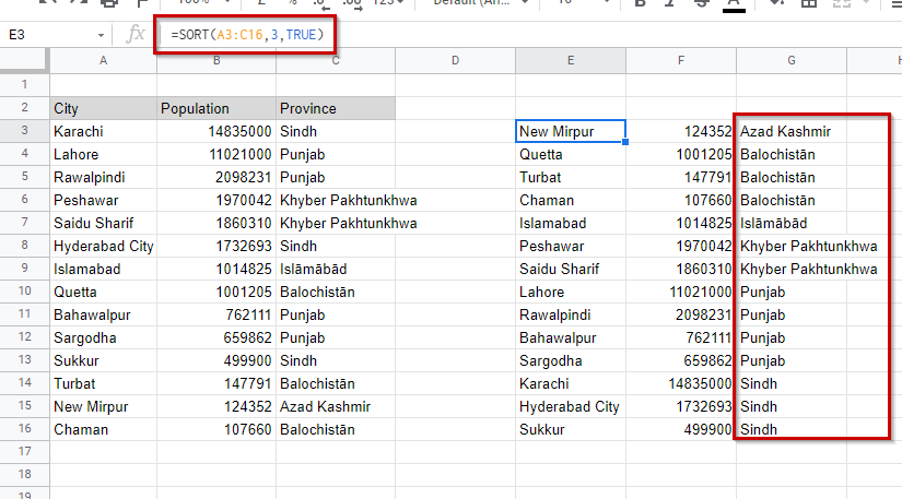
In order to arrange the data according to provinces, simply change the index number, from the above example to 3. The formula becomes.
=SORT(A3:C16,3,TRUE)
and the resulting table will be:
How to Alphabetize in Google Sheets Based on a Column not Included inside the DataSet?
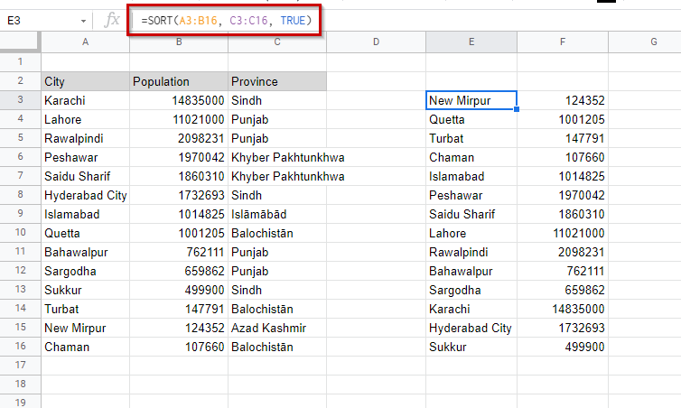
Now, if we don’t want the list of provinces to be included in our sorted table, but do want the data sorted according to the provinces, then, our range will be A3:B16, leaving out the list of provinces that will now be indexed in sort_column in the formula.
So, the formula, in this case, will become:
=SORT(A3:B16,C3:C16,TRUE)
Press enter to get the final result. The result here will display the cities in order, according to the provinces, without displaying the actual list of the provinces itself.
If we had written “FALSE” instead of “TRUE” here, in the above formula, google sheets would’ve returned the same data but in descending (reverse-alphabetical) order.
2. How to Alphabetize in Google Sheets Using the Built-In Option
Besides through the SORT function, the data can be organized using the Google Sheets built-in sort option too. This option gives static, fixed values that cannot be changed, unlike the dynamic results that the SORT function gives, and is only suitable if you’re not regularly updating your data.
Here’s how to alphabetize in Google Sheets using the built-in sort options available. Let’s take only the cities here, as our example.
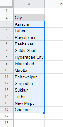
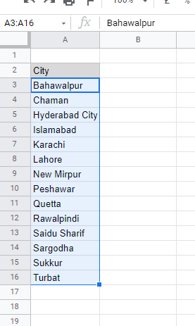
As the first step, you need to select your data set. Our data set is A3 to A16.
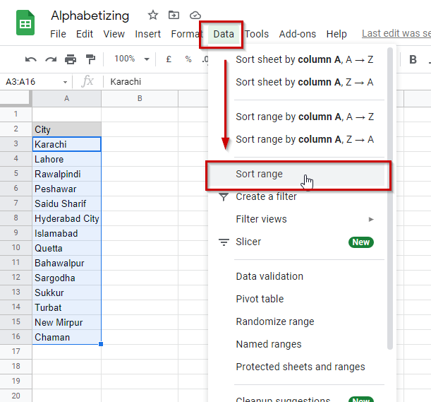
Now, go to “Data” from the menu bar, and then, from the dropdown menu select “Sort range”.
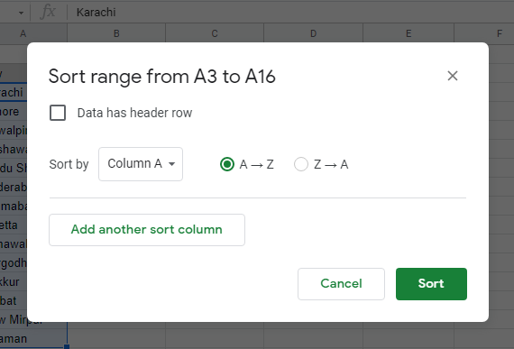
A pop-up will appear.
We will keep the “Data has header row” option unchecked as our original selection did not include the header cell A2 that reads “City”. If the selection range was A2:A16, this box would have to be checked to avoid getting the A2 cell getting sorted, too. This is an important thing to confirm before sorting the data.
The next option “Sort by” is to be used in case of a range with multiple columns as this option allows you to select which column will be the one to sort the rest of the selection according to.
Out of the two options available, “A → Z” sorts in ascending order, whereas, “Z → A”, if selected, will sort the data in descending order.
Adding other sorting columns allows users to add to the range.
Once the desired settings have been applied, all you need to do is to click on “Sort”. Google Sheets will then display the final result.
How to Alphabetize in Google Sheets on a Smartphone?
Just like on a desktop, data can be sorted on Google Sheets on a mobile phone screen too. Here are all the steps involved in how to alphabetize in Google Sheets when using a smartphone:
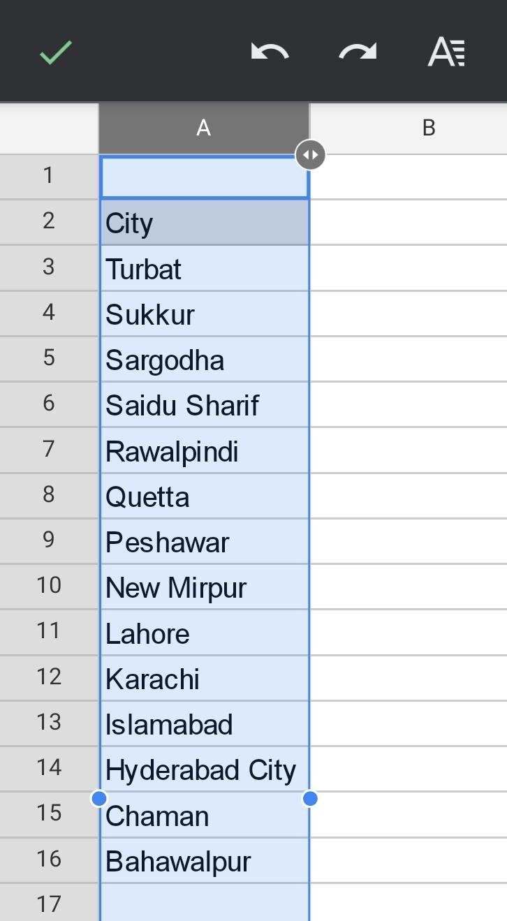
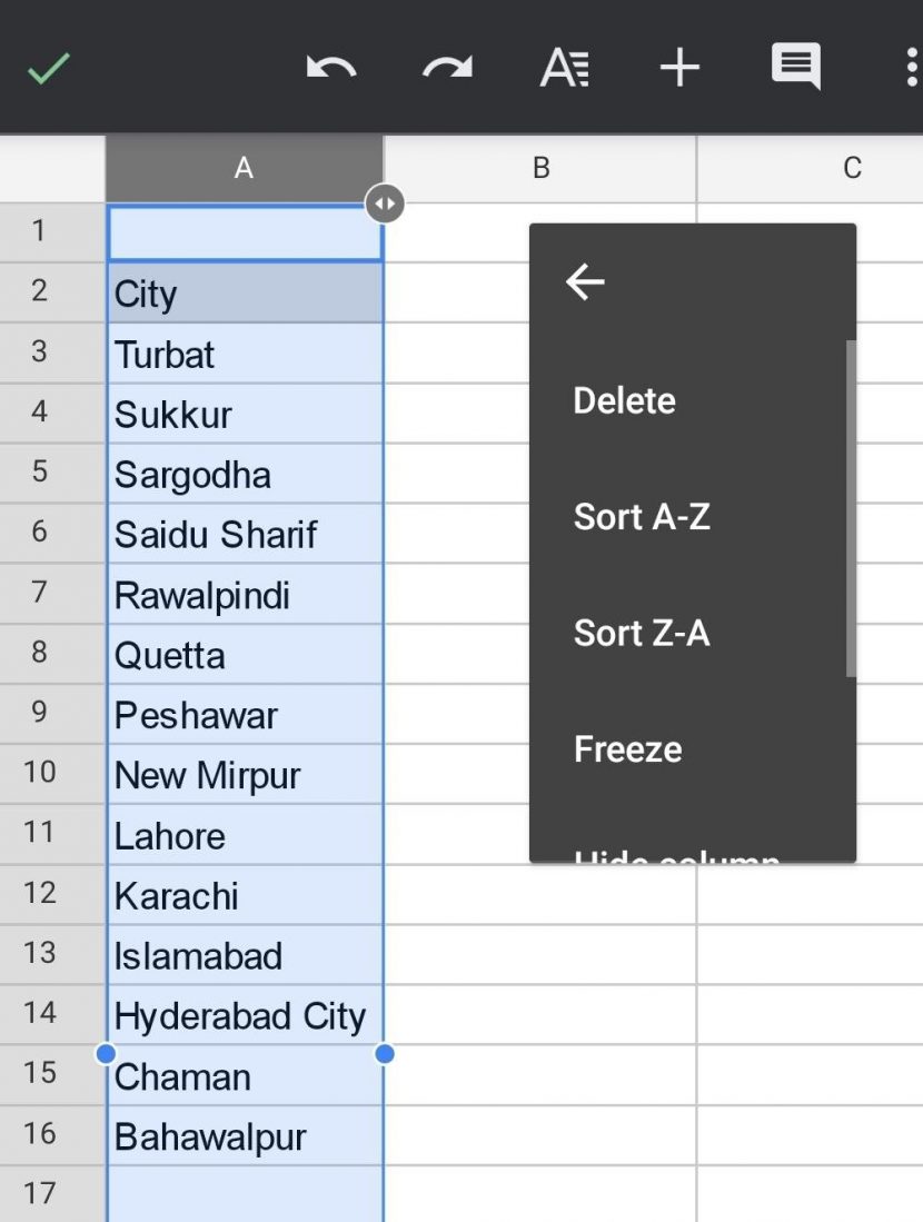
Let’s begin by establishing our data. Following is our dataset on a mobile phone:
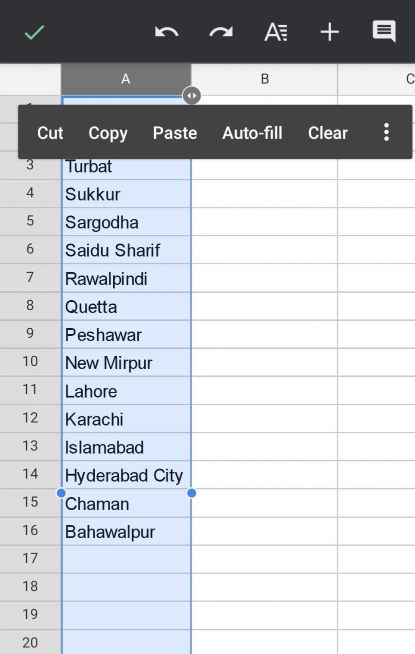
Click on the top of this column where the column title “A” is mentioned. Once the entire column is selected, tap it again. When tapped the second time, a small list of options will appear.
From here, click on the right-most option that shows three dots in a column. This will display another set of options that offer both A – Z and Z – A sorting for the cells in the selected column.
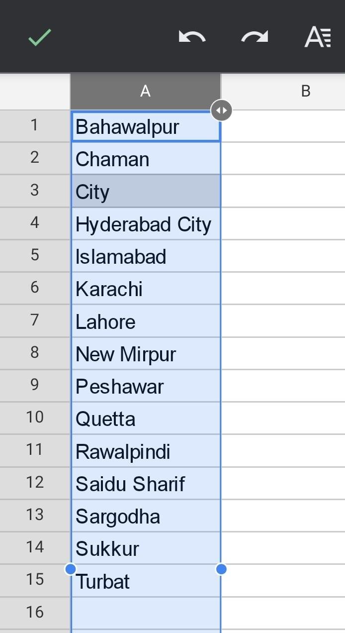
Here, we will click on “A – Z” to get our data sorted in ascending order.
Here, the only catch is that the whole column is selected only and your header can also get shuffled. To avoid this issue you can simply first order the cells and add the header later, or adjust it after sorting.
Sorting in google sheets is very simple, and if you understand even the simplest “SORT function” method, you can easily arrange as much data as you want to.
